The usual approach to Euler deconvolution using a moving window scheme produces a lot of spurious solutions. This is expected because we are running the deconvolution once per window for the whole area. We don’t specify the number of sources that we expect and the deconvolution doesn’t give us that information.
An alternate approach is to use an expanding window scheme. It runs the deconvolution on a number of windows expanding from a given central point. We choose only one of the solutions as the final estimate (the one with the smallest error). This approach will give you a single solution. You can interpret multiple bodies by selecting multiple expanding window centers, one for each anomaly.
The expanding window scheme is implemented in
fatiando.gravmag.euler.EulerDeconvEW.
Out:
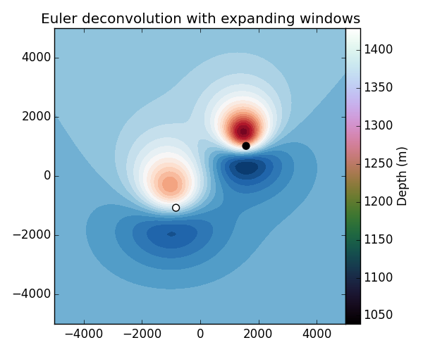
Euler solutions:
Lower right anomaly location: [-1072.04297339  -830.29615323  1428.85976886]
Upper left anomaly location: [ 1018.12838822  1576.71821498  1039.07466633]
Centers of the model spheres:
[-1000 -1000  1500]
[1000 1500 1000]
from __future__ import print_function
from fatiando.gravmag import sphere, transform, euler
from fatiando import gridder, utils, mesher
import matplotlib.pyplot as plt
import numpy as np

# Make some synthetic magnetic data to test our Euler deconvolution.
# The regional field
inc, dec = -45, 0
# Make a model of two spheres magnetized by induction only
model = [
    mesher.Sphere(x=-1000, y=-1000, z=1500, radius=1000,
                  props={'magnetization': utils.ang2vec(2, inc, dec)}),
    mesher.Sphere(x=1000, y=1500, z=1000, radius=1000,
                  props={'magnetization': utils.ang2vec(1, inc, dec)})]
# Generate some magnetic data from the model
shape = (100, 100)
area = [-5000, 5000, -5000, 5000]
x, y, z = gridder.regular(area, shape, z=-150)
data = sphere.tf(x, y, z, model, inc, dec)

# We also need the derivatives of our data
xderiv = transform.derivx(x, y, data, shape)
yderiv = transform.derivy(x, y, data, shape)
zderiv = transform.derivz(x, y, data, shape)

# Now we can run our Euler deconv solver using expanding windows. We'll run 2
# solvers, each one expanding windows from points close to the anomalies.

# We use a structural index of 3 to indicate that we think the sources are
# spheres.

# Make the solver and use fit() to obtain the estimate for the lower right
# anomaly
print("Euler solutions:")
sol1 = euler.EulerDeconvEW(x, y, z, data, xderiv, yderiv, zderiv,
                           structural_index=3, center=(-2000, -2000),
                           sizes=np.linspace(300, 7000, 20))
sol1.fit()
print("Lower right anomaly location:", sol1.estimate_)

# Now run again for the other anomaly
sol2 = euler.EulerDeconvEW(x, y, z, data, xderiv, yderiv, zderiv,
                           structural_index=3, center=(2000, 2000),
                           sizes=np.linspace(300, 7000, 20))
sol2.fit()
print("Upper left anomaly location:", sol2.estimate_)

print("Centers of the model spheres:")
print(model[0].center)
print(model[1].center)

# Plot the solutions on top of the magnetic data. Remember that the true depths
# of the center of these sources is 1500 m and 1000 m.

plt.figure(figsize=(6, 5))
plt.title('Euler deconvolution with expanding windows')
plt.contourf(y.reshape(shape), x.reshape(shape), data.reshape(shape), 30,
             cmap="RdBu_r")
plt.scatter([sol1.estimate_[1], sol2.estimate_[1]],
            [sol1.estimate_[0], sol2.estimate_[0]],
            c=[sol1.estimate_[2], sol2.estimate_[2]],
            s=50, cmap='cubehelix')
plt.colorbar(pad=0).set_label('Depth (m)')
plt.xlim(area[2:])
plt.ylim(area[:2])
plt.tight_layout()
plt.show()

# A cool thing about this scheme is that the window centers do not have to fall
# on the middle of the anomaly for it to work.
Total running time of the script: ( 0 minutes 0.243 seconds)