Euler deconvolution attempts to estimate the coordinates of simple (idealized) sources from the input potential field data. There is a strong assumption that the sources have simple geometries, like spheres, vertical pipes, vertical planes, etc. So it wouldn’t be much of a surprise if the solutions aren’t great when sources are complex.
Let’s test the Euler deconvolution using a moving window scheme, a very common
approach used in all industry software. This is implemented in
fatiando.gravmag.euler.EulerDeconvMW.
Out:
Centers of the model spheres:
[-1000 -1000  1500]
[1000 1500 1000]
Kept Euler solutions after the moving window scheme:
[[ 1005.02117863  1555.11042642   998.68593456]
 [ 1042.92870628  1479.25104857   982.8034785 ]
 [ -903.03736426  -826.2551998   1580.03357152]
 [ -996.30379977  -940.33986512  1459.01039032]
 [ 1159.1957134   1006.77185575  1199.42292819]
 [ 1465.17965473   408.39773001  1920.31472105]
 [  991.40325194  1468.18742261  1020.67590594]
 [ -966.01139554  -775.38064946  1465.22351287]
 [-1041.3450269   -971.09938734  1500.22185195]
 [ -284.04967711  -382.06786678  2243.58685856]
 [  -35.58602726  -108.90046998  1540.68712849]
 [ 1058.8441761   1516.37801553   994.86866767]
 [  999.08320679  1580.06304764  1051.97367365]
 [ -933.90137199  -995.14775353  1406.97615438]
 [  381.76290333  1131.68128707   992.51158521]
 [  914.43334205  1475.15646829   978.0510579 ]
 [ 1277.82392557  1876.41150747   931.05131937]
 [-1017.82794862 -1140.04437429  1560.46288409]
 [ -991.58404782 -1012.73293178  1556.74635058]
 [ -349.91796733   355.56106336  1792.13495774]]
from __future__ import print_function
from fatiando.gravmag import sphere, transform, euler
from fatiando import gridder, utils, mesher
import matplotlib.pyplot as plt
# Make some synthetic magnetic data to test our Euler deconvolution.
# The regional field
inc, dec = -45, 0
# Make a model of two spheres magnetized by induction only
model = [
mesher.Sphere(x=-1000, y=-1000, z=1500, radius=1000,
props={'magnetization': utils.ang2vec(2, inc, dec)}),
mesher.Sphere(x=1000, y=1500, z=1000, radius=1000,
props={'magnetization': utils.ang2vec(1, inc, dec)})]
print("Centers of the model spheres:")
print(model[0].center)
print(model[1].center)
# Generate some magnetic data from the model
shape = (100, 100)
area = [-5000, 5000, -5000, 5000]
x, y, z = gridder.regular(area, shape, z=-150)
data = sphere.tf(x, y, z, model, inc, dec)
# We also need the derivatives of our data
xderiv = transform.derivx(x, y, data, shape)
yderiv = transform.derivy(x, y, data, shape)
zderiv = transform.derivz(x, y, data, shape)
# Now we can run our Euler deconv solver on a moving window over the data.
# Each window will produce an estimated point for the source.
# We use a structural index of 3 to indicate that we think the sources are
# spheres.
# Run the Euler deconvolution on moving windows to produce a set of solutions
# by running the solver on 10 x 10 windows of size 1000 x 1000 m
solver = euler.EulerDeconvMW(x, y, z, data, xderiv, yderiv, zderiv,
structural_index=3, windows=(10, 10),
size=(1000, 1000))
# Use the fit() method to obtain the estimates
solver.fit()
# The estimated positions are stored as a list of [x, y, z] coordinates
# (actually a 2D numpy array)
print('Kept Euler solutions after the moving window scheme:')
print(solver.estimate_)
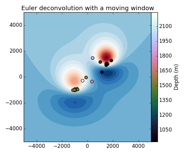
# Plot the solutions on top of the magnetic data. Remember that the true depths
# of the center of these sources is 1500 m and 1000 m.
plt.figure(figsize=(6, 5))
plt.title('Euler deconvolution with a moving window')
plt.contourf(y.reshape(shape), x.reshape(shape), data.reshape(shape), 30,
cmap="RdBu_r")
plt.scatter(solver.estimate_[:, 1], solver.estimate_[:, 0],
s=50, c=solver.estimate_[:, 2], cmap='cubehelix')
plt.colorbar(pad=0).set_label('Depth (m)')
plt.xlim(area[2:])
plt.ylim(area[:2])
plt.tight_layout()
plt.show()
Total running time of the script: ( 0 minutes 0.220 seconds)