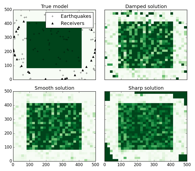
A very simplified way of playing around with tomography is through a straight-ray approximation. If we assume that the seismic rays don’t bend when they encounter a change in velocity (i.e., no refraction), then the inversion becomes linear and much simpler to solve. It is a good example to illustrate how different forms of regularization impact the estimated velocity model.
This simple tomography is implemented in the
SRTomo class. The example below uses 3 forms
of regularization to invert a synthetic data-set.
import numpy as np
import matplotlib.pyplot as plt
from fatiando.mesher import SquareMesh
from fatiando.seismic import ttime2d, srtomo
from fatiando.inversion import Smoothness2D, Damping, TotalVariation2D
from fatiando import utils, gridder

# First, we'll create a simple model with a high velocity square in the middle
area = (0, 500000, 0, 500000)
shape = (30, 30)
model = SquareMesh(area, shape)
vel = 4000 * np.ones(shape)
vel[5:25, 5:25] = 10000
model.addprop('vp', vel.ravel())

# Make some noisy travel time data using straight-rays
# Set the random seed so that points are the same every time we run this script
seed = 0
src_loc_x, src_loc_y = gridder.scatter(area, 80, seed=seed)
src_loc = np.transpose([src_loc_x, src_loc_y])
rec_loc_x, rec_loc_y = gridder.circular_scatter(area, 30,
                                                random=True, seed=seed)
rec_loc = np.transpose([rec_loc_x, rec_loc_y])
srcs = [src for src in src_loc for _ in rec_loc]
recs = [rec for _ in src_loc for rec in rec_loc]
tts = ttime2d.straight(model, 'vp', srcs, recs)
# Use 2% random noise to corrupt the data
tts = utils.contaminate(tts, 0.02, percent=True, seed=seed)

# Make a mesh for the inversion. The inversion will estimate the velocity in
# each square of the mesh. To make things simpler, we'll use a mesh that is the
# same as our original model.
mesh = SquareMesh(area, shape)

# Create solvers for each type of regularization and fit the synthetic data to
# obtain an estimated velocity model
solver = srtomo.SRTomo(tts, srcs, recs, mesh)

smooth = solver + 1e8*Smoothness2D(mesh.shape)
smooth.fit()

damped = solver + 1e8*Damping(mesh.size)
damped.fit()

sharp = solver + 30*TotalVariation2D(1e-10, mesh.shape)
# Since Total Variation is a non-linear regularizing function, then the
# tomography becomes non-linear as well. We need to configure the inversion to
# use the Levemberg-Marquardt algorithm, a gradient descent method, that
# requires an initial estimate
sharp.config('levmarq', initial=0.00001*np.ones(mesh.size)).fit()

# Plot the original model and the 3 estimates using the same color bar
fig, axes = plt.subplots(2, 2, figsize=(8, 7), sharex='all', sharey='all')

x = model.get_xs()/1000
y = model.get_ys()/1000
vmin, vmax = vel.min(), vel.max()

ax = axes[0, 0]
ax.set_title('True model')
ax.pcolormesh(x, y, vel, cmap='Greens', vmin=vmin, vmax=vmax)
ax.plot(src_loc[:, 0]/1000, src_loc[:, 1]/1000, '+k', label='Earthquakes')
ax.plot(rec_loc[:, 0]/1000, rec_loc[:, 1]/1000, '^k', label='Receivers')
ax.legend(loc='upper right', numpoints=1)

ax = axes[0, 1]
ax.set_title('Damped solution')
ax.pcolormesh(x, y, damped.estimate_.reshape(shape), cmap='Greens', vmin=vmin,
              vmax=vmax)

ax = axes[1, 0]
ax.set_title('Smooth solution')
ax.pcolormesh(x, y, smooth.estimate_.reshape(shape), cmap='Greens', vmin=vmin,
              vmax=vmax)

ax = axes[1, 1]
ax.set_title('Sharp solution')
ax.pcolormesh(x, y, sharp.estimate_.reshape(shape), cmap='Greens', vmin=vmin,
              vmax=vmax)

plt.tight_layout()
plt.show()
Total running time of the script: ( 0 minutes 4.459 seconds)