Synthetic seismograms using the convolutional model¶

import numpy as np
import matplotlib.pyplot as plt
from fatiando.seismic import conv
from fatiando.vis import mpl

# Define the parameters of our depth model
n_samples, n_traces = [600, 100]
velocity = 1500*np.ones((n_samples, n_traces))
# We'll put two interfaces in depth
velocity[150:, :] = 2000
velocity[400:, :] = 3500

# We need to convert the depth model we made above into time
vel_l = conv.depth_2_time(velocity, velocity, dt=2e-3, dz=1)
# and we'll assume the density is homogeneous
rho_l = 2200*np.ones(np.shape(vel_l))
# With that, we can calculate the reflectivity model in time
rc = conv.reflectivity(vel_l, rho_l)
# and finally perform our convolution
synt = conv.convolutional_model(rc, 30, conv.rickerwave, dt=2e-3)

# We can use the utility function in fatiando.vis.mpl to plot the seismogram
fig, axes = plt.subplots(1, 2, figsize=(8, 5))

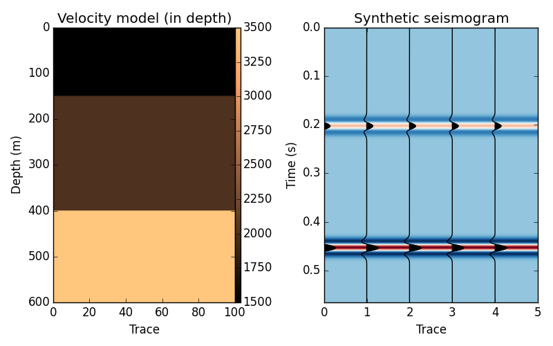
ax = axes[0]
ax.set_title("Velocity model (in depth)")
tmp = ax.imshow(velocity, extent=[0, n_traces, n_samples, 0],
                cmap="copper", aspect='auto', origin='upper')
fig.colorbar(tmp, ax=ax, pad=0, aspect=50)
ax.set_xlabel('Trace')
ax.set_ylabel('Depth (m)')

ax = axes[1]
ax.set_title("Synthetic seismogram")
mpl.seismic_wiggle(synt[:, ::20], dt=2.e-3, scale=1)
mpl.seismic_image(synt, dt=2.e-3, cmap="RdBu_r", aspect='auto')
ax.set_xlabel('Trace')
ax.set_ylabel('Time (s)')
plt.tight_layout()
plt.show()