The equivalent layer is one of the best methods for griding and upward continuing gravity data and much more. The trade-off is that performing this requires an inversion and later forward modeling, which are more time consuming and more difficult to tune than the standard griding and FFT-based approaches.
This example uses the equivalent layer in fatiando.gravmag.eqlayer to
grid and upward continue some gravity data. There are more advanced methods in
the module than the one we are showing here. They can be more efficient but
usually require more configuration.
Out:
Residuals:
  mean: 0.0246019125949 mGal
  stddev: 0.179200376563 mGal
from __future__ import division, print_function
import matplotlib.pyplot as plt
from fatiando.gravmag import prism, sphere
from fatiando.gravmag.eqlayer import EQLGravity
from fatiando.inversion import Damping
from fatiando import gridder, utils, mesher
# First thing to do is make some synthetic data to test the method. We'll use a
# single prism to keep it simple
props = {'density': 500}
model = [mesher.Prism(-5000, 5000, -200, 200, 100, 4000, props)]
# The synthetic data will be generated on a random scatter of points
area = [-8000, 8000, -5000, 5000]
x, y, z = gridder.scatter(area, 300, z=0, seed=42)
# Generate some noisy data from our model
gz = utils.contaminate(prism.gz(x, y, z, model), 0.2, seed=0)
# Now for the equivalent layer. We must setup a layer of point masses where
# we'll estimate a density distribution that fits our synthetic data
layer = mesher.PointGrid(area, 500, (20, 20))
# Estimate the density using enough damping so that won't try to fit the error
eql = EQLGravity(x, y, z, gz, layer) + 1e-22*Damping(layer.size)
eql.fit()
# Now we add the estimated densities to our layer
layer.addprop('density', eql.estimate_)
# and print some statistics of how well the estimated layer fits the data
residuals = eql[0].residuals()
print("Residuals:")
print(" mean:", residuals.mean(), 'mGal')
print(" stddev:", residuals.std(), 'mGal')
# Now I can forward model gravity data anywhere we want. For interpolation, we
# calculate it on a grid. For upward continuation, at a greater height. We can
# even combine both into a single operation.
x2, y2, z2 = gridder.regular(area, (50, 50), z=-1000)
gz_up = sphere.gz(x2, y2, z2, layer)
fig, axes = plt.subplots(1, 2, figsize=(8, 6))
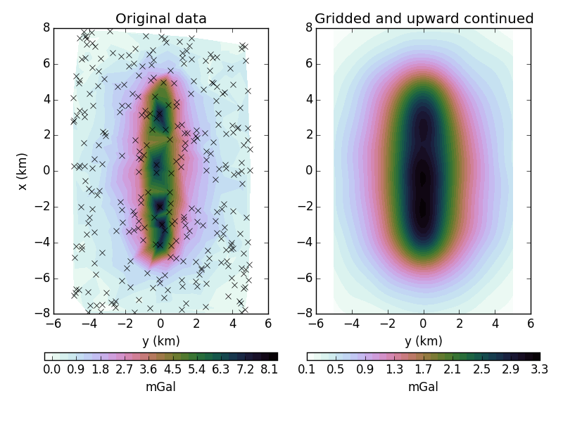
ax = axes[0]
ax.set_title('Original data')
ax.set_aspect('equal')
tmp = ax.tricontourf(y/1000, x/1000, gz, 30, cmap='cubehelix_r')
fig.colorbar(tmp, ax=ax, pad=0.1, aspect=30,
orientation='horizontal').set_label('mGal')
ax.plot(y/1000, x/1000, 'xk')
ax.set_xlabel('y (km)')
ax.set_ylabel('x (km)')
ax = axes[1]
ax.set_title('Gridded and upward continued')
ax.set_aspect('equal')
tmp = ax.tricontourf(y2/1000, x2/1000, gz_up, 30, cmap='cubehelix_r')
fig.colorbar(tmp, ax=ax, pad=0.1, aspect=30,
orientation='horizontal').set_label('mGal')
ax.set_xlabel('y (km)')
plt.tight_layout()
plt.show()
Total running time of the script: ( 0 minutes 0.524 seconds)