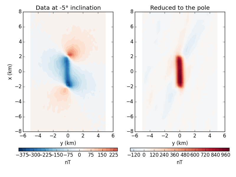
Equivalent layer for reduction to the pole of magnetic data¶

The equivalent layer can be used to reduce magnetic data to the pole. One of the main advantages of this approach over the FFT based reduction if that the equivalent layer doesn’t suffer from instabilities at low latitudes.

However, both the FFT algorithm (fatiando.gravmag.transform.reduce_to_pole) and the equivalent layer required the knowing the total magnetization direction of the anomaly source. If the there is only induced magnetization, this will be the direction of the Earth’s field. But if there is also remanent magnetization or any self-demagnetizing effects, then the direction will be different. One method for estimating the total magnetization direction is through fatiando.gravmag.magdir.DipoleMagDir if the anomaly source is approximately spherical.

This example uses the equivalent layer in fatiando.gravmag.eqlayer to grid and reduce to the pole some magnetic data. There are more advanced methods in the module than the one we are showing here. They can be more efficient but usually require more configuration.

../../_images/sphx_glr_eqlayer_mag_transform_001.png

Out:

Residuals:
  mean: -0.0472055944107 nT
  stddev: 4.74326555726 nT

from __future__ import division, print_function
import matplotlib.pyplot as plt
import numpy as np
from fatiando.gravmag import prism, sphere
from fatiando.gravmag.eqlayer import EQLTotalField
from fatiando.inversion import Damping
from fatiando import gridder, utils, mesher

# First thing to do is make some synthetic data to test the method. We'll use a
# single prism with only induced magnetization to keep it simple
inc, dec = -5, 23
props = {'magnetization': utils.ang2vec(5, inc, dec)}
model = [mesher.Prism(-2000, 2000, -200, 200, 100, 4000, props)]

# The synthetic data will be generated on a regular grid
area = [-8000, 8000, -5000, 5000]
shape = (40, 40)
x, y, z = gridder.regular(area, shape, z=-150)
# Generate some noisy data from our model
data = utils.contaminate(prism.tf(x, y, z, model, inc, dec), 5, seed=0)

# Now for the equivalent layer. We must setup a layer of dipoles where we'll
# estimate a magnetization intensity distribution that fits our synthetic data.
# Notice that we only estimate the intensity. We must provide the magnetization
# direction of the layer through the sinc and sdec parameters.
layer = mesher.PointGrid(area, 700, shape)
eql = (EQLTotalField(x, y, z, data, inc, dec, layer, sinc=inc, sdec=dec)
       + 1e-15*Damping(layer.size))
eql.fit()
# Print some statistics of how well the estimated layer fits the data
residuals = eql[0].residuals()
print("Residuals:")
print("  mean:", residuals.mean(), 'nT')
print("  stddev:", residuals.std(), 'nT')

# Now I can forward model data anywhere we want. To reduce to the pole, we must
# provide inc = 90 (or -90) for the Earth's field as well as to the layer's
# magnetization.
layer.addprop('magnetization', utils.ang2vec(eql.estimate_, inc=-90, dec=0))
atpole = sphere.tf(x, y, z, layer, inc=-90, dec=0)


fig, axes = plt.subplots(1, 2, figsize=(8, 6))

ax = axes[0]
ax.set_title(u'Data at {}° inclination'.format(inc))
ax.set_aspect('equal')
amp = np.abs([data.min(), data.max()]).max()
tmp = ax.tricontourf(y/1000, x/1000, data, 30, cmap='RdBu_r', vmin=-amp,
                     vmax=amp)
fig.colorbar(tmp, ax=ax, pad=0.1, aspect=30,
             orientation='horizontal').set_label('nT')
ax.set_xlabel('y (km)')
ax.set_ylabel('x (km)')

ax = axes[1]
ax.set_title('Reduced to the pole')
ax.set_aspect('equal')
amp = np.abs([atpole.min(), atpole.max()]).max()
tmp = ax.tricontourf(y/1000, x/1000, atpole, 30, cmap='RdBu_r', vmin=-amp,
                     vmax=amp)
fig.colorbar(tmp, ax=ax, pad=0.1, aspect=30,
             orientation='horizontal').set_label('nT')
ax.set_xlabel('y (km)')

plt.tight_layout()
plt.show()

Total running time of the script: ( 0 minutes 2.257 seconds)

Generated by Sphinx-Gallery